IEEE TRANSACTIONS ON ROBOTICS, VOL. 39, NO. 6, DECEMBER 2023 4805 Aerobatic Trajectory Generation for a VTOL Fixed-Wing Aircraft Using Differential Flatness Ezra Tal , Gilhyun Ryou , and Sertac Karaman , Member, IEEE Abstract—This article proposes a novel algorithm for aerobatic trajectory generation for a vertical take-off and landing (VTOL) tailsitter flying wing aircraft. The algorithm differs from existing approaches for fixed-wing trajectory generation, as it considers a realistic six-degree-of-freedom (6-DOF) flight dynamics model, including aerodynamic equations. Using a global dynamics model enables the generation of aerobatics trajectories that exploit the entire flight envelope, allowing agile maneuvering through the stall regime, sideways uncoordinated flight, inverted flight, etc. The method uses the differential flatness property of the global tailsitter flying wing dynamics, which is derived in this work. By performing snap minimization in the differentially flat output space, a compu- tationally efficient algorithm, suitable for online motion planning, is obtained. The algorithm is demonstrated in extensive flight ex- periments encompassing six aerobatic maneuvers, a time-optimal drone racing trajectory, and an airshowlike aerobatic sequence for three tailsitter aircraft. Index Terms—Aerial systems, autonomous vehicle navigation, mechanics and control, motion and path planning, trajectory optimization. I. INTRODUCTION V ERTICAL take-off and landing (VTOL) fixed-wing air- craft combine many of the advantages traditionally asso- ciated with either fixed-wing aircraft or rotorcraft. They can ex- ceed the range and endurance limitations typical of multicopters, while maintaining the capability to take-off, hover, and land in confined spaces. This versatility is relevant to many real-world applications. For example, transitioning search and rescue air- craft can cover large areas efficiently and closely inspect (indoor) areas of particular interest. Similarly, VTOL delivery drones can safely make time-critical deliveries in remote environments without the need for a dedicated landing area. Tailsitter VTOL aircraft transition between hover and for- ward flight by pitching, so that their rotors transition between lift generation and forward propulsion based on the attitude. The tailsitter flying wing omits a tail and vertical surfaces, Manuscript received 17 May 2023; accepted 20 July 2023. Date of publication 18 August 2023; date of current version 6 December 2023. This paper was recom- mended for publication by Associate Editor Hector Garcia de Marina and Editor Paolo Robuffo Giordano upon evaluation of the reviewers’ comments. This work was supported by the Army Research Office under Grant W911NF1910322. (Corresponding author: Ezra Tal.) The authors are with the Laboratory for Information and Decision Systems, Massachusetts Institute of Technology, Cambridge, MA 02139 USA (e-mail: eatal@mit.edu; ghryou@mit.edu; sertac@mit.edu). This article has supplementary material provided by the au- thors and color versions of one or more figures available at https://doi.org/10.1109/TRO.2023.3301312. Digital Object Identifier 10.1109/TRO.2023.3301312 Fig. 1. Loop trajectory reference and flight experiment. leading to a relatively simple mechanical design consisting of just a wing, two rotors, and two flaps that function as both elevators and ailerons. By placing these flaps in the rotor wash and using differential thrust, the aircraft remains controllable throughout the flight envelope, including static conditions. The simple, lightweight design allows a high thrust-to-weight ra- tio and the absence of a vertical tail surface reduces direc- tional stability, leading to a highly agile and maneuverable aircraft. In this article, we show that, under some assumptions, the tailsitter flying wing flight dynamics are differentially flat. This entails that the state and input variables can be expressed as a function of a flat output and a finite number of its deriva- tives [1], [2]. Based on this flatness transform, we propose an algorithm for generating fast and agile tailsitter trajectories with low computational cost, i.e., suitable for online motion planning applications. Our algorithm is capable of generating aerobatic maneuvers that exploit the entire flight envelope of the vehicle, including challenging conditions, such as sideways knife-edge flight and inverted flight, as shown in Fig. 1. Existing trajectory generation algorithms for fixed-wing air- craft often avoid the relatively complicated flight dynamics and instead use kinematics models. For example, an extension of Dubins paths can be used to find the time-optimal trajectory with curvature constraints [3]. While accurate tracking of the resulting paths is not dynamically feasible due to the instanta- neous acceleration changes needed to transition between straight lines and circular arcs, feedback control can be used to maintain © 2023 The Authors. This work is licensed under a Creative Commons Attribution-NonCommercial-NoDerivatives 4.0 License. For more information, see https://creativecommons.org/licenses/by-nc-nd/4.0/ 4806 IEEE TRANSACTIONS ON ROBOTICS, VOL. 39, NO. 6, DECEMBER 2023 a tracking error that is acceptable in calm flight [4]. When con- sidering fast and agile flight, the aircraft dynamics and control input constraints must be considered in trajectory generation, so that the resulting trajectory is dynamically feasible, i.e., so that it can be accurately tracked in flight. Trajectory optimization subject to the six-degree-of-freedom (6-DOF) nonlinear flight dynamics model is computationally costly, e.g., optimization of the 4.5 m knife-edge maneuver presented by [5] takes 3–5 min of computation time (using direct collocation with twelve states and five control inputs) according to [6]. Existing work addresses computational expense in various ways, e.g., by considering only (extended) point-mass equations of motion [7], [8], [9], by using a planner with precomputed maneuvers [10], [11], by incorporating human-piloted expert demonstrations [12], or by combining multiple simplified local dynamics models [13]. In practice, these methods may impose limitations on the generated trajectories, especially when planning aerobatic maneuvers that rapidly progress through unconventional flight conditions. In the context of trajectory generation, differential flatness enables the transformation of trajectories from the flat output space to the state and control input space [1], [14]. This property is widely leveraged toward computationally efficient trajectory generation and tracking for quadcopters by defining the trajec- tory in the flat output space consisting of the 3-D position and the yaw angle [15], [16], [17]. Differential flatness of fixed-wing aircraft dynamics has also been considered [14]. However, the application of differential flatness toward trajectory generation for fixed-wing aircraft has mostly been limited to kinematics or simplified dynamics models. Existing works consider path generation and tracking using a differentially flat coordinated flight model [18] and aerobatic maneuvers using an aircraft kinematics model that does not incorporate an angle of attack or sideslip angle [19]. The algorithm presented in [6] is based on the differentially flat coordinated flight model given in [18] and combines Dubins paths with a transverse polynomial offset to obtain smooth trajectories. Our proposed method differs from existing flatness-based approaches for fixed-wing trajectory generation, as it consid- ers a global 6-DOF flight dynamics model, including aero- dynamic equations. By using a global dynamics model, we are able to generate aerobatic maneuvers that exploit the en- tire flight envelope, enabling agile maneuvering through the stall regime, sideways uncoordinated flight, inverted flight, etc. As we will show, the tailsitter flatness transform has a simi- lar structure as the well-known quadcopter flat transform, in the sense that snap and yaw acceleration roughly correspond to the control inputs. Hence, their reduction also increases the feasibility of tailsitter trajectories, akin to the premise of minimum-snap trajectory generation algorithms for quad- copters [15], [16]. This enables the application of similar ef- ficient algorithms for minimum-snap trajectory generation in the flat output space toward generation of tailsitter aerobatic trajectories. Our work contains several contributions. First, we propose an algorithm for aerobatic trajectory generation for a VTOL fixed-wing aircraft using differential flatness. As far as we are aware, this is the first algorithm that uses differential flatness of a realistic fixed-wing flight dynamics model to generate aer- obatic flight trajectories. Second, we show differential flatness of the tailsitter flying wing dynamics model. We computation- ally and experimentally validate the suitability of the derived flatness transform to determine dynamic feasibility of candidate trajectories. Third, we provide extensive experimental results encompassing trajectories and flight tests for: 1) six aerobatics maneuvers; 2) a time-optimal drone racing trajectory at the limit of the vehicle’s capability; 3) an airshowlike aerobatic sequence for three tailsitter aircraft. We note that our recent work on trajectory-tracking tailsitter flight control [20] also leverages differential flatness of the global flight dynamics model. While both works consider aerobatic trajectories, they address funda- mentally different problems. Where [20] considers the control problem, i.e., the calculation of the closed-loop control inputs that enable the vehicle to accurately fly a commanded trajectory; the current work considers motion planning, i.e., the generation of reference trajectories subject to the physical constraints of the vehicle and the environment. These problems are complemen- tary, i.e., the controller derived in [20] may be used to track the trajectories generated by the algorithms presented in the current work. Finally, we note that [20] does not include a method to obtain the open-loop control inputs as a function of the higher order output derivatives, including snap and yaw acceleration, which is necessary for trajectory generation. The rest of this article is organized as follows. Section II presents preliminaries on the tailsitter flying wing flight dynam- ics and on minimum-snap trajectory generation. The tailsitter flying wing flatness transform is derived in Section III and its suitability to predict the dynamic feasibility of candidate trajectories is assessed in Section IV. Section V contains gener- ated trajectories and experimental flight results for aggressive aerobatic maneuvers, a racing trajectory, and a multivehicle aerobatic sequence. Finally, Section VI concludes this article. II. PRELIMINARIES A. Flight Dynamics In this section, we provide a brief overview of the tailsitter flight dynamics model from [20] as a preliminary to the deriva- tion of the corresponding flatness transform in Section III, which forms the basis of our trajectory generation algorithm. 1) Vehicle Equations of Motion: The vehicle translational dynamics are given by ˙x = v (1) ˙v = giz + m−1Ri αf α (2) where x and v are, respectively, the vehicle position and ve- locity in the world-fixed reference frame, g is the gravitational acceleration, and m is the vehicle mass. The vector f α represents the aerodynamic and thrust force in the vehicle-fixed zero-lift reference frame, shown in Fig. 2(a). This frame is obtained by rotating the body-fixed axis system, shown in Fig. 2(b), around its negative by-axis by the zero-lift angle of attack α0, which is defined as the angle of attack for which the aircraft produces zero lift. The body-fixed frame itself is defined by the wing TAL et al.: AEROBATIC TRAJECTORY GENERATION FOR A VTOL FIXED-WING AIRCRAFT 4807 Fig. 2. Reference frame and control input conventions. The green board is mounted toward the top of the wing; the yellow battery toward its bottom. (a) Zero-lift reference frame α, zero-lift angle of attack α0, and thrust angle αT . (b) Body-fixed reference frame b, and control inputs, i.e., rotor speeds ω1 and ω2, and flap deflections δ1 and δ2. chord line and symmetry plane. The origin of both frames is at the center of the mass. The transformation matrix Ri α represents the orientation of the zero-lift axis system with regard to the local north-east-down (NED) world-fixed reference frame, which we will indicate with the columns of the identity matrix [ix iy iz]. The rotational dynamics are given by ˙ξ = 1 2 ξ ◦ Ω (3) ˙Ω = J−1(m − Ω × JΩ) (4) where Ω is the angular velocity in the body-fixed reference frame, and ξ is the unit quaternion attitude vector. The matrix J is the vehicle moment of inertia tensor, and m represents the aerodynamic and thrust moment in the body-fixed reference frame. 2) Force and Moment: The following equations, due to [20], employ the ϕ-theory parameterization by [21] to obtain a global singularity-free model of the aerodynamic force and moment. The force in the zero-lift axis system is obtained by summing contributions from thrust, flaps, and wings, as follows: f α = f α T + f α δ + f α w. (5) The thrust force is given by f α T = 2∑ i=1 ⎡ ⎣ cos ¯α (1 − cDT ) 0 sin ¯α (cLT − 1) ⎤ ⎦ Ti ︸ ︷︷ ︸ f α Ti (6) where ¯α is the angle of the thrust line with regard to the zero-lift axis, i.e., ¯α = α0 + αT , Ti is the thrust due to motor i, and the dimensionless coefficients cDT and cLT represent, respectively, the loss of propeller efficiency due to the presence of the wing in the propwash and the propwash-induced lift. The motor thrust is computed as follows: Ti = cT ω2 i with i = 1, 2 (7) where cT is the thrust coefficient in kg·m/rad2 (or equivalently N/(rad/s)2) and ωi ≥ 0 is the speed of motor i. We note that the quadratic approximation (7) is sufficiently accurate at the relatively low speeds achieved in indoor flight, but that high speed outdoor flight may warrant a more sophisticated thrust model, as remarked in [20]. The force contribution by the flaps is given by f α δ = 2∑ i=1 − ⎡ ⎣ 0 0 cδ LT cos ¯α Ti + cδ LV ‖v‖i� x vα ⎤ ⎦ δi ︸ ︷︷ ︸ f α δi (8) where δi is the deflection angle of flap i, the dimensionless parameter cδ LT represents the propwash-induced flap force, and cδ LV (in kg/m) corresponds to the flap force due to the movement of the wing through the surrounding air. Finally, the wing force contribution is obtained as f α w = − ⎡ ⎢ ⎣ cDV i� x vα 0 cLV i� z vα ⎤ ⎥ ⎦ ‖v‖ (9) where the parameters cDV and cLV in kg/m represent, respec- tively, drag and lift acting on the wing due to its movement through the air. We note that (5) does not contain any lateral force component, due to the absence of a fuselage and vertical tail surface. Similarly, we obtain the moment in the body-fixed reference frame by summing contributions due to the motor thrust and torque and the flap deflections m = mT + mμ + mδ. (10) The moment due to motor thrust is given by mT = ⎡ ⎢ ⎣ lTy i� z Rb α(f α T2 − f α T1) cμT (T1 + T2) lTy i� x Rb α(f α T1 − f α T2) ⎤ ⎥ ⎦ (11) 4808 IEEE TRANSACTIONS ON ROBOTICS, VOL. 39, NO. 6, DECEMBER 2023 where lTy is the moment arm with regard to the center of gravity and cμT represents the thrust-induced pitch moment, akin to a moment arm. The moment due to motor torque is obtained as follows: mμ = ⎡ ⎢ ⎣ cos αT 0 − sin αT ⎤ ⎥ ⎦ 2∑ i=1 μi (12) where μi = −(−1)icμω2 i with i = 1, 2 (13) is the motor torque around the thrust-axis with cμ the propeller torque coefficient in kg·m2/rad2 (or equivalently N·m/(rad/s)2). The flap contribution is given by mδ = ⎡ ⎢ ⎣ lδy cos α0 i� z (f α δ2 − f α δ1) lδxi� z (f α δ1 + f α δ2) lδy sin α0 i� z (f α δ2 − f α δ1) ⎤ ⎥ ⎦ (14) where lδy and lδx are the relevant moment arms. Moment contributions due to the freestream velocity and the angular velocity are neglected, as most of these are relatively small for the tailless flying wing and their inclusion may result in a much more complicated expression for the flatness transform. An evaluation of the impact of modeling assumptions is provided in Section IV. Note that all aerodynamic coefficients incorporate the air density. If significantly varying conditions are incurred, their values can be adjusted by scaling with air density. The interested reader is referred to [20] for an analytical deriva- tion of the coefficients, including a comparison to conventional (Buckingham-π) fixed-wing aerodynamic coefficients. B. Minimum-Snap Trajectory Generation As we will show in Section III, the tailsitter dynamics model— with some simplifications—admits a differentially flat output σ(t) = [x(t)� ψ(t)]� (15) consisting of four elements: the vehicle position in the world- fixed reference frame x(t) ∈ R3, and the yaw angle (which is formally defined in Section III-A) ψ(t) ∈ T, where T denotes the circle group. Consequently, any sufficiently smooth output trajectory satisfies the dynamics (1)–(4) and, conversely, any state-space trajectory (including aerobatic trajectories with un- conventional flight conditions) corresponds to a unique output trajectory (15). This bijective correspondence can be exploited to generate dynamically feasible aerobatics trajectories without resorting to computationally expensive state-space methods. When focusing on aggressive flight trajectories, generation is complicated by the fact that the control input constraints, i.e., the motor speed and flap deflection limits, cannot readily be enforced in the flat output space. Widely used algorithms for trajectory generation in the differentially flat output space of the quadcopter dynamics address this difficulty by minimizing snap, i.e., the fourth derivative of position, and yaw acceleration [15]. In practice, this optimization roughly corresponds to reducing the required control moment and thus increasing the likelihood that the control input limits are satisfied and the trajectory is feasible. In Section III, we show that the flatness transform for the tailsitter dynamics has a similar form with control inputs depending on snap and yaw acceleration. This makes snap minimization also suitable for generating aggressive tailsitter trajectories. Elementary minimum-snap optimization subject to waypoint constraints can be formulated as follows: minimize σ ∫ T 0 ∥ ∥ ∥ ∥ d4x dt4 ∥ ∥ ∥ ∥ 2 + μψ ( d2ψ dt2 )2 dt subject to σ ⎛ ⎝ i∑ j=1 tj ⎞ ⎠ = ˜σi, i = 0, . . . , m (16) where μψ is a weighing parameter. The nonnegative vector t rep- resents the time allocation over the trajectory segments between the m + 1 waypoints ˜σ that must be attained in order. Minimum- snap trajectory generation for quadcopters is widely studied, and various methods to obtain t have been proposed [15], [16], [22]. In principle, our framework for flatness-based trajectory generation is detached from the exact optimization formulation, enabling it to profit from the extensive research on minimum- snap trajectory generation, including extensions such as obstacle avoidance [23]. In this article, we use the formulation by [16] to describe the trajectory with piecewise polynomial functions that we define in terms of their derivatives at the waypoints. For a given time allocation t, the corresponding minimum-snap trajectory is then efficiently obtained in closed form using matrix multiplications, which we conveniently denote as σ = χ (t, ˜σ, ˙˜σ, ¨˜σ, . . . ) (17) where ˙˜σ, ¨˜σ etc. denote optional derivative constraints that may be set at some of the waypoints. We first minimize snap subject to a rough estimate ¯T of the total trajectory time based on the distance between waypoints, as follows: minimize σ,t ∫ ¯T 0 ∥ ∥ ∥ ∥ d4x dt4 ∥ ∥ ∥ ∥ 2 + μψ ( d2ψ dt2 )2 dt subject to σ = χ (t, ˜σ, ˙˜σ, ¨˜σ, . . . ) m∑ j=1 tj = ¯T . (18) In order to obtain aggressive aerobatic trajectories, we then minimize the scale factor c that is applied to the resulting time allocation t. As such, we obtain the quickest minimum-snap trajectory σ = χ(ct, ˜σ, ˙˜σ, ¨˜σ, . . . ) that is in the feasible set ΣT = { σ ∣ ∣ ∣u(t) ∈ U ∀t ∈ [0, T ] } (19) where u is the control input trajectory corresponding to σ and U is the set of permissible control inputs, i.e., the bounded set defined by the minimum and maximum allowed rotor speeds and flap deflections. We perform the minimization of c using a bijection method with multiple initialization points, where feasibility of each candidate solution is evaluated using (19). In TAL et al.: AEROBATIC TRAJECTORY GENERATION FOR A VTOL FIXED-WING AIRCRAFT 4809 addition to minimum-snap optimization, we employ the method described in [22] to optimize the time allocation t using exper- imental evaluations, as described in Section V-B. III. DIFFERENTIAL FLATNESS TRANSFORM In recent work on tailsitter flight control, we have shown how the vehicle attitude and angular velocity can be obtained based on the trajectory (15) and its derivatives up to yaw rate and jerk (i.e., the third derivative of position) [20]. In this section, we extend this derivation to obtain the full differential flatness transform, including an expression for the control inputs based on the trajectory derivatives up to yaw acceleration and snap. This expression enables us to verify that the motor speeds and flap deflections corresponding to a candidate trajectory are permissible, i.e., that the trajectory is in the feasible set (19). A. Attitude We first derive expressions for the attitude and collective thrust. Rewriting (2) as f i = m (a − giz) (20) shows that the vehicle attitude and collective thrust are uniquely defined by three major constraints: i) the yaw angle ψ; ii) the fact that i� y f α = 0 according to (5); iii) the forces in the vehicle symmetry plane, i.e., i� x f α and i� z f α. The Euler angles ψ, φ, and θ in ZXY rotation sequence are used to describe the attitude of the body-fixed frame shown in Fig. 2(b) with regard to the world-fixed NED frame, such that ψ = φ = θ = 0 indicates wings-level forward flight toward the north. As we will show in this section, these angles form a valid and universal attitude representation with each angle defined by one of the three constraints given above. The angle symbols are also used to refer to the intermediate frames up to and including the corresponding rotation, such that, e.g., f b = Rb i f i = Rb φRφ ψRψ i f i, where f b is expressed in the body- fixed frame and f i in the world-fixed frame. The first Euler rotation is the yaw rotation ψiz, such that the angle between the direction of the right wingtip, i.e., by, and the world-fixed east-axis iy equals ψ. As the subsequent roll and pitch rotations do not affect the horizontal component of by, the angle between iy and the horizontal projection of the wingtip remains ψ. This definition of yaw—based on the wingtip rather than the nose direction—has the advantage that yaw is well- defined in both forward flight and hover. Yaw is only undefined in the less common condition of 90° roll, which is addressed below. Next, constraint (ii) is satisfied by the roll rotation φ = − atan2 ( i� y Rψ i f i, i� z f i) + kπ (21) around the yawed x-axis Ri ψix, where atan2 is the four-quadrant inverse tangent function. Constraint (ii) is satisfied ∀k ∈ {0, 1} and, in practice, k can be set such that the obtained attitude trajectory is continuous. We note that rotation through the Eu- ler angle singularity at |φ| = π/2 rad causes the yaw angle to switch to ψ + π for very large roll angles. When incurring this condition, we avoid discontinuities by considering ψ and ψ + π rad equivalent, so that k in (21) can be set freely to enforce attitude continuity. In practice, permitting yaw switching to ψ + π enables aggressive maneuvers such as turns with over 90° banking angle. Any unwanted switching is avoided by virtue of the smoothness constraints imposed on σ, described at the end of Section III-C. Finally, constraint (iii) is satisfied by equating (5) and (20) and solving for the collective thrust T = T1 + T2 and for the pitch rotation angle ¯θ from the frame φ to the zero-lift reference frame. In solving these equations, we neglect the nonminimum phase dynamics due to the direct force contribution by the flaps. When combined with feedback control, this approach achieves good trajectory generation and tracking performance for slightly nonminimum phase systems [24]. The method is simple and avoids the large and quickly changing control actions that ex- act feedback linearization of the nonminimum phase system may result in [25]. We note that potentially a flat output of the nonminimum phase dynamics could be used to guarantee stable tracking [26]. However, this approach requires defining the trajectory in terms of the center of oscillation instead of the vehicle center of mass, leading to difficulty with the relatively complicated 6-DOF tailsitter dynamics model. We substitute f α = R¯θ φf φ with f φ = Rφ i f i as well as a similar expression for vα into (5) to obtain c¯α (1 − cDT ) T − cDV ‖v‖ (c¯θ i� x vφ − s¯θ i� z vφ) = c¯θ i� x f φ − s¯θ i� z f φ (22) s¯α (cLT − 1)T − cLV ‖v‖ (s¯θ i� x vφ + c¯θ i� z vφ) = s¯θ i� x f φ + c¯θ i� z f φ (23) where c and s represent cosine and sine, respectively. Solving (22) and (23) for ¯θ and T gives ¯θ = atan2 ( η (i� x f φ + cDV ‖v‖i� x vφ) − cLV ‖v‖i� z vφ − i� z f φ η (i� z f φ + cDV ‖v‖i� z vφ) + cLV ‖v‖i� x vφ + i� x f φ ) + kπ (24) T = 1 c¯α (1 − cDT ) ( c¯θ i� x f φ − s¯θ i� z f φ + cDV ‖v‖ ( c¯θ i� x vφ − s¯θ i� z vφ )) (25) where η = s¯α (cLT − 1) c¯α (1 − cDT ) (26) is the ratio of lift and forward force due to thrust. Again, the constraint is satisfied ∀k ∈ {0, 1} and, in practice, k can be set such that the obtained attitude trajectory is continuous. Finally, 4810 IEEE TRANSACTIONS ON ROBOTICS, VOL. 39, NO. 6, DECEMBER 2023 the pitch rotation of the body-fixed reference frame is obtained as θ = ¯θ + α0. B. Angular Velocity An expression for the angular velocity is obtained by taking the derivative of the Euler angles. From (21), we obtain ˙φ = − ˙βxβz − βx ˙βz β2 x + β2 z (27) where βx and βz are, respectively, the first and second arguments of the atan2 function, and ˙βx = − cψ ˙ψi� x f i − sψ i� x ˙f i − sψ ˙ψi� y f i + cψ i� y ˙f i (28) ˙βz = i� z ˙f i (29) with, from the derivative of (20) ˙f i = mj (30) where j indicates the jerk, i.e., the third temporal derivative of position. Similarly, from (24) we obtain ˙θ = ˙σxσz − σx ˙σz σ2 x + σ2 z (31) where σx and σz are the respective arguments of the atan2 function, and ˙σx = η ( i� x ˙f φ + cDV τx ) − cLV τz − i� z ˙f φ (32) ˙σz = η ( i� z ˙f φ + cDV τz ) + cLV τx + i� x ˙f φ (33) with τx = ˙‖v‖i� x vφ + ‖v‖i� x ˙vφ (34) τz = ˙‖v‖i� z vφ + ‖v‖i� z ˙vφ (35) and ˙‖v‖ = v�a ‖v‖ (36) ˙vφ = ˙Rφ i v + Rφ i a. (37) The expression for the force derivative ˙f φ is similar to (37). As described in Section III-A, we neglect the direct force contribu- tion by the flaps. Finally, we obtain the angular velocity in the body-fixed reference frame, as follows: Ω = ⎡ ⎣ 0 ˙θ 0 ⎤ ⎦ + Rθ φ ⎡ ⎣ ˙φ 0 0 ⎤ ⎦ + Rθ ψ ⎡ ⎣ 0 0 ˙ψ ⎤ ⎦ . (38) C. Motor Speeds and Flap Deflections In order to obtain the control inputs, we first derive an expression for the angular acceleration as a function of snap and yaw acceleration. By taking the derivative of (27), we obtain the following expression for the roll acceleration: ¨φ = (β2 x + β2 z )−2 (( ˙βxβz − βx ˙βz ) ( 2βx ˙βx + 2βz ˙βz ) − ( ¨βxβz − βx ¨βz ) (β2 x + β2 z )) (39) where ¨βx = ( sψ ˙ψ2 − cψ ¨ψ ) i� x f i − 2 cψ ˙ψi� x ˙f i − sψ i� x ¨f i − ( cψ ˙ψ2 + sψ ¨ψ ) i� y f i − 2 sψ ˙ψi� y ˙f i + cψ i� y ¨f i (40) ¨βz = i� z ¨f i (41) are obtained as the derivatives of (28) and (29), and the second force derivative is a function of the snap s, i.e., ¨f i = ms. (42) Similarly, by taking the derivative of (31) we obtain the pitch acceleration ¨θ = ((¨σxσz − σx ¨σz) (σ2 x + σ2 z ) − ( ˙σxσz − σx ˙σz) (2σx ˙σx + 2σz ˙σz)) (σ2 x + σ2 z )−2 (43) where ¨σx = η ( i� x ¨f φ + cDV ˙τx ) − cLV ˙τz − i� z ¨f φ (44) ¨σz = η ( i� z ¨f φ + cDV ˙τz ) + cLV ˙τx + i� x ¨f φ (45) with ˙τx = ¨‖v‖i� x vφ + 2 ˙‖v‖i� x ˙vφ + ‖v‖i� x ¨vφ (46) ˙τz = ¨‖v‖i� z vφ + 2 ˙‖v‖i� z ˙vφ + ‖v‖i� z ¨vφ (47) and ¨‖v‖ = a�a + v�j ‖v‖ − v�a ˙‖v‖ ‖v‖2 (48) ¨vφ = ¨Rφ i v + 2 ˙Rφ i a + Rφ i j. (49) The expression for the force second derivative ¨f φ is similar to (49). We combine the roll acceleration and pitch acceleration ob- tained from respectively (39) and (43) with the yaw acceleration ¨ψ to obtain the angular acceleration in the body-fixed reference frame. We take the derivative of (38) to obtain the following expression: ˙Ω = ⎡ ⎣ 0 ¨θ 0 ⎤ ⎦ + ˙Rθ φ ⎡ ⎣ ˙φ 0 0 ⎤ ⎦ + Rθ φ ⎡ ⎣ ¨φ 0 0 ⎤ ⎦ + ˙Rθ ψ ⎡ ⎣ 0 0 ˙ψ ⎤ ⎦ + Rθ ψ ⎡ ⎣ 0 0 ¨ψ ⎤ ⎦ . (50) TAL et al.: AEROBATIC TRAJECTORY GENERATION FOR A VTOL FIXED-WING AIRCRAFT 4811 We can now find the moment in the body-fixed reference frame by rewriting (4), as follows: m = J ˙Ω + Ω × JΩ. (51) Next, we solve (10) for the flap deflections and differential thrust ΔT = T1 − T2. We find an expression for ΔT by equating i� z (mT + mμ) = i� z m (52) which assumes that the contribution by i� z mδ is negligible. Due to the multiplication with sin α0, this assumption typically does not result in significant discrepancies. Using μ1 + μ2 = cμ/cT ΔT , we obtain ΔT = i� z m ( − sαT cμ cT + lTy (cα0 c¯α (1 − cDT ) − sα0 s¯α (cLT − 1)) )−1 . (53) The individual thrust values are then given by T1 = T + ΔT 2 , T2 = T − ΔT 2 (54) and the motor speeds can be obtained from (7). For the flap deflections, we deduct mT and mμ from m to obtain mδ, and we rewrite (14), as follows: [δ1 δ2 ] = [−lδy cα0 ν1 lδy cα0 ν2 lδxν1 lδxν2 ]−1 [i� x mδ i� y mδ ] (55) with νi = −cδ LT cos ¯α Ti − cδ LV ‖v‖i� x vα. (56) Note that—since the control inputs cannot instantaneously change—dynamic feasibility of σ requires continuity of (51), and therefore at least fourth-order continuity of the position x and at least second-order continuity of the yaw ψ. IV. DYNAMIC FEASIBILITY We classify a trajectory as dynamically feasible if it can be flown, i.e., tracked, by the actual vehicle within a specified error bound. Concretely, we define the set of feasible trajectories over the time interval [0, T ] as ΣT = { σ ∣ ∣ ∣‖xref (t) − x(t)‖ < ¯x ∧ |ψref (t) − ψ(t)| < ¯ψ ∀t ∈ [0, T ] } (57) where ¯x and ¯ψ are the error bounds on position and yaw tracking, respectively. In practice, these error bounds may be applied as safety margins when flying around obstacles, so that collisions are avoided. Evaluation of (57) is challenging in reality, since it needs to account for the entire system, including flight dynamics, actuation and control systems, sensing and state estimation etc. Instead, we resort to (19), which classifies a trajectory as feasible if the corresponding open-loop control inputs are permissible, i.e., within the bounded set defined by the minimum and maxi- mum allowed rotor speeds and flap deflections. Intuitively, this Fig. 3. 6 m hover-to-hover trajectory with ψstart = 0 rad, ψend = π rad. Trajectory time is 3 s, interval between poses is 0.25 s. means that there exists a permissible open-loop control input that makes the ideal, deterministic vehicle model perfectly track the entire trajectory. In this section, we evaluate (57) through flight experiments and we evaluate (19) using the flatness transform. By comparing the results, we evaluate the suitability of the flat- ness transform presented in Section III to determine feasibility of a candidate trajectory on the actual vehicle. A description of the experimental setup is given in Section V. A. Hover-to-Hover Trajectory We consider a single-segment hover-to-hover trajectory with ˜σ0 = [0 0 0 ψstart]� (58) ˜σ1 = [6 [m] 0 0 ψend]� . (59) This trajectory requires large acceleration and simultaneous yawing motion through the transition regime. Based on the flatness transform described in Section III, we determine the minimal feasible time for the minimum-snap trajectory with various ψstart and ψend. An example trajectory is shown in Fig. 3. Fig. 4 shows results for the trajectory with yawing motion from ψstart to ψend using the minimal rotation. It can be seen that the fastest times are achieved in the center of the figure, around ψstart = ψend = 0 rad, which corresponds to forward coordinated flight. We observe discontinuity along the yaw direction switching lines, which indicates that the interplay between translational and yaw dynamics may render it beneficial to yaw in the opposite direction, e.g., traversing more than 180° in order to avoid inverted flight. However, in practice the difference is typically small, meaning that the min- imal rotation that is obtained from optimization in the flat out- put space—where this interplay is not considered—is (nearly) optimal. We conduct experiments to compare the feasibility boundary from Fig. 4 to the tracking error of the actual vehicle. Fig. 5 shows the tracking error for the hover-to-hover trajectory in coordinated flight without yaw, i.e., ψstart = ψend = 0 rad, and for the same trajectory but with ψstart = 0 rad, ψend = π rad. Each point on 4812 IEEE TRANSACTIONS ON ROBOTICS, VOL. 39, NO. 6, DECEMBER 2023 Fig. 4. Minimum feasible time for 6 m hover-to-hover trajectory using mini- mal yaw rotation. the curves corresponds to a flight experiment. As the trajectory time on the horizontal axis increases, the maneuvers become less aggressive, and the tracking error decreases. The corresponding feasibility boundaries predicted in Fig. 4 are indicated by the colored shading, i.e., the shaded areas in the left of the figure correspond to infeasible trajectory times. While only a single color is shown at a time, the infeasibility areas continue from their boundary all the way to the vertical axis on the left. For the yawing trajectory, the tracking error increases at lower speeds compared to the coordinated flight trajectory, as predicted by the feasibility boundaries. We note that these boundaries correspond to the most aggressive trajectories that theoretically can be tracked by the given vehicle dynamics model, neglecting practical factors such as modeling errors and imperfect state estimation and control, so that it is expected that significant tracking error occurs before they are reached. The coordinated flight trajectory at the feasibility boundary (2.0 s) attains a maximum speed of 7.6 m/s within 1 s and attains a maximum load of 3.1 g. It is tracked with less than 1 m position tracking error. B. Circular Trajectory In order to evaluate the accuracy of the feasibility prediction at high speed and large sustained acceleration, we use the flat- ness transform to determine the maximum speed on a circular trajectory with a 3 m radius. As shown in Fig. 6, we consider two trimmed conditions, coordinated and knife-edge flight, as well as a rolling/yawing motion where ψ changes at the same rate but in the opposite direction. The position and yaw derivatives for evaluation of the feasibility are given in Table I. We perform experiments for all three circular trajectories at various speeds. The results are shown in Fig. 7, where each point on the curves corresponds to a flight experiment. The figure is oriented similarly to Fig. 5 with the most aggressive, i.e., the highest speed, trajectories toward the left. It shows that the flat dynamics model predicts that coordinated flight can be performed up to the highest speed, followed by knife-edge flight, and finally, the rolling circle, which has a relatively low TABLE I FLAT OUTPUT (DERIVATIVES) FOR VARIOUS CIRCULAR TRAJECTORIES WITH Ω = v/r maximum speed. The position tracking errors obtained from flight experiments agree with this prediction. Fig. 7(a) shows the expected increase in each position tracking error before the corresponding shaded area is reached. Similar behavior can be observed in Fig. 7(b) for the yaw tracking error on the coordinated and rolling circle. The yaw error in knife-edge flight remains very small, even at high speeds, because—in this condition—the vehicle orientation reduces the sensitivity of yaw to attitude errors and increases the yaw control effectiveness by differential thrust. Since the flat transform does not consider lateral forces on the tailless aircraft, the speed in circular knife-edge flight is mostly limited by the maximum thrust. In fact, completely neglecting the aerodynamics and solving for the maximum speed vmax = √ 2cT ¯ω2 r m (60) with ¯ω the maximum motor speed, results in only a small overestimation when compared to the maximum speed obtained from the flat transform (9.5 m/s versus 9.2 m/s). In flight ex- periments, the vehicle achieved RMS position and yaw tracking errors of respectively 12.5 cm and 1.1° at 8 m/s, approaching the theoretical maximum speed with relatively small track- ing error. Considering that at least some control input mar- gin must be maintained to enable stabilization of the unstable knife-edge condition (making the theoretical limit unattain- able), this affirms that the lateral aerodynamic force must in- deed be quite small and can be neglected in the flat dynamics model. Considering the comparative results for both trajectories, we can conclude that the differential flatness transform gives a useful prediction of the critical trajectory time or speed where we can expect to observe a stark increase in tracking error on the real vehicle. V. FLIGHT EXPERIMENTS We present extensive experimental results to validate the generated aerobatic trajectories. These flight tests demonstrate six types of aerobatic maneuvers, a racing trajectory through a sequence of gates, and an airshowlike aerobatic sequence with three aircraft that aggressively maneuver in close proximity to obstacles and to each other. Video of the experiments can be found in the supplementary materials. The 3-D-printed tailsitter used for the experiments is shown in Fig. 8. Detailed description of its design and manufacturing can TAL et al.: AEROBATIC TRAJECTORY GENERATION FOR A VTOL FIXED-WING AIRCRAFT 4813 Fig. 5. Tracking error in flight experiments 6 m hover-to-hover trajectory. Shaded area indicates infeasibility according to differential flatness transform. (a) Maximum position tracking error with and without yaw rotation. (b) Maximum yaw tracking error with and without yaw rotation. Fig. 6. Circular trajectory with various yaw references. (a) Coordinated. (b) Knife edge. (c) Rolling. Fig. 7. Tracking error in flight experiments for circular trajectory with various yaw references. Shaded area indicates infeasibility according to differential flatness transform. (a) RMS position tracking error. (b) RMS yaw tracking error. Fig. 8. Tailsitter flying wing aircraft used in the experiments. be found in [27]. Table II lists key aircraft properties, including aerodynamic parameters that were estimated using flight data. The drag parameters cDV and cDT are set to zero, because their estimation is impractical in the limited space of our indoor fight room, as described in [20]. As described in Section II-B, our algorithm uses the flatness transform to generate the state and control input trajectory. The resulting open-loop control inputs are only used to evaluate feasibility of the candidate trajectory and not for flight control. Only the instantaneous trajectory reference σ(t) and its deriva- tives, i.e., the current reference position, velocity, acceleration, jerk, yaw, and yaw rate, are provided to the control system by the trajectory generation algorithm. Based on these reference signals and the current state estimate, the controller computes the closed-loop control inputs that are sent to the motors and flap servos. We refer the interested reader to [20] for a detailed description of the control system. 4814 IEEE TRANSACTIONS ON ROBOTICS, VOL. 39, NO. 6, DECEMBER 2023 Fig. 9. Loop. Interval between poses is 0.7 s. (a) Reference with waypoints. Start and end points are static hover, and arrows indicate velocity direction constraints. (b) Experiment. Fig. 10. Loop trajectory at various speeds. Shaded areas indicate infeasibility according to the differential flatness transform and coincide with increased experimental tracking error. (a) Maximum flap deflection and motor speed according to the differential flatness transform. Dashed lines indicate vehicle limits. (b) Maximum position tracking error in flight experiments. TABLE II TAILSITTER AIRCRAFT PROPERTIES A. Aerobatic Maneuvers We first demonstrate how the flatness transform enables gen- eration of aerobatic maneuvers using relatively simple waypoint (derivative) constraints in the trajectory output space. The result- ing maneuvers exploit the full flight envelope of the tailsitter aircraft, including poststall and sideways flight, and do not require restrictive assumptions such as coordinated flight and curvature limitations. The data shown in Table III confirms the aerobatic character of the trajectories, which reach speeds up to 8.0 m/s, loads of over 3 g, and angular rates that exceed 650°/s. Conforming to the observations from Section IV, we found that each maneuver can be slowed down to reduce tracking error but we chose to accept some tracking error in favor of increased aggressiveness. 1) Loop: The loop trajectory shown in Fig. 9 consists of five waypoints (of which two coincide) on a vertical circle with 1 m radius, and start and end points constrained to static hover. We add tangential velocity constraints to enforce a circular path. As shown in Fig. 10, the loop trajectory has several feasibility boundaries. When flown slowly (i.e., below 2.5 m/s), the tra- jectory is feasible and flown in hover attitude with θ ≈ π/2 rad. When flown faster (i.e., around 4.5 m/s), the vehicle performs a loop, making a full upward pitch rotation. Intermediate speeds (i.e., around 3 m/s) are too slow to perform a loop and require the vehicle to quickly pitch back down at the top of the circular segment, rendering the trajectory infeasible due to flap deflec- tion limits, as shown in Fig. 10(a). Fig. 10(b) shows that the maximum position tracking error obtained from flight experi- ments shows a corresponding stark increase in this region of infeasibility. Increasing the speed to 5.2 m/s requires ever larger TAL et al.: AEROBATIC TRAJECTORY GENERATION FOR A VTOL FIXED-WING AIRCRAFT 4815 TABLE III MAXIMUM SPEED, LOAD, AND ANGULAR RATE FOR REFERENCE TRAJECTORIES; AND MAXIMUM AND ROOT MEAN SQUARE (RMS) POSITION TRACKING ERROR FOR FLIGHT EXPERIMENTS Fig. 11. Coordinated to knife-edge to coordinated flight. Interval between poses is 0.6 s. (a) Reference with waypoints. Start and end points are static hover, and arrows indicate 5 m/s velocity constraints. (b) Experiment. Fig. 12. Climbing turn with 1 m height difference. Interval between poses is 0.5 s. (a) Reference with waypoints. Start and end points are static hover, and arrows indicate 5 m/s velocity constraints. (b) Experiment. acceleration, ultimately leading to infeasibility due to motor speed limitations. Fig. 10(a) shows that this limitation is ap- proached more gradually, which also leads to a more gradual in- crease in tracking error in Fig. 10(b). The trajectory with a max- imum speed of 3.8 m/s is shown in Fig. 9. The loop maneuver is successfully performed in the flight experiment. The maximum position error of 74 cm is incurred when exiting the final circular segment. 2) Knife-Edge Flight: Fig. 11 shows a straight trajectory between static hover start and end points. The intermediate waypoints enforce a constant speed of 5 m/s and serve to transition between flight attitudes through the yaw reference ψref . In the first of the three middle segments, the vehicle transitions from coordinated to knife-edge fight; in the second, it maintains constant knife-edge orientation; and in the third, it transitions back to coordinated flight. Performing the transitions while maintaining straight flight at 5 m/s is challenging due to the aerodynamic interactions between vehicle attitude, flap deflections, and rotor speeds. As expected, the position tracking error in the flight experiment increases at the transitions. Once knife-edge orientation is reached, the position tracking error quickly reduces again. The vehicle attitude during knife-edge flight differs somewhat between the reference and experiment trajectories. The increased pitch angle in the experiment compensates for the neglected flap force contribution, and the small rotation toward the direction of travel compensates for the nonzero lateral force. Finally, we note that the largest position tracking error is incurred close to the end point. This error is mainly along the trajectory and is caused by delayed deceleration. The maximum path error, i.e., position error with regard to the closest point on the trajectory line, occurs during the second transition and amounts to 47 cm. 3) Climbing Turn: We plan a climbing turn trajectory using four waypoints, as shown in Fig. 12. The start and end points are constrained to static hover, and the two intermediate waypoints are positioned with only a height difference. Using velocity 4816 IEEE TRANSACTIONS ON ROBOTICS, VOL. 39, NO. 6, DECEMBER 2023 Fig. 13. Immelmann turn. Interval between poses is 1.0 s. (a) Reference with waypoints. Start and end points are static hover, and arrows indicate 6 m/s velocity constraints. (b) Experiment. Fig. 14. Split S maneuver. Interval between poses is 1.0 s. (a) Reference with waypoints. Start and end points are static hover, and arrows indicate 5 m/s velocity constraints. (b) Experiment. constraints, we enforce straight and coordinated flight at these intermediate waypoints. Hence, the entire 270° turn and 1 m climb occur between these two waypoints. During the turn, the reference trajectory reaches about 90° banking angle, requires nearly the maximum motor speeds of 2500 rad/s, and reaches a peak angular rate of 11.3 rad/s (647°/s). A peak load of 3.1 g is required during the turn, while the loads close to the start and end points reach up to 2.0 g. Consequently, the vehicle quickly completes the 11.3 m trajectory in 3.1 s, despite starting and ending in static hover. In the flight experiment, we observe that, during the turn, a maximum load of 3.4 g and a peak angular rate of 10.9 rad/s (625°/s) are attained. The motors briefly saturate, resulting in some loss of altitude. Once the saturation is resolved, the vehicle quickly catches up and reduces the position tracking error to below 20 cm before the turn is exited. 4) Immelmann Turn: The Immelmann turn is a well-known aerobatics and aerial combat maneuver that reverses direction by performing a half loop followed by a half roll, as shown in Fig. 13. We generate the trajectory using static hover start and end points, and four intermediate waypoints. The intermediate waypoints enforce constant speed coordinated flight prior to the half loop and constant speed transition from inverted to regular coordinated flight afterward. Similar to the loop and knife-edge maneuvers described above, we observe increased error when exiting the loop segment, increased error during transition through uncoordinated flight orientation, and delayed deceleration toward the end point. Comparison of the vehicle poses also leads to similar observations of small differences: increased pitch to account for flap force and increased yaw in uncoordinated flight to compensate for the nonzero lateral force. The Immelmann turn combines several challenging aspects to exploit the expansive flight envelope of the tailsitter vehicle. The maneuver contains large accelerations, inverted flight, and a transition through the entire yaw range (i.e., from ψref = 0 to ψref = ±π rad) at a peak angular rate of 9.4 rad/s (538°/s) while maintaining a linear speed of 6 m/s. Based on snap minimization and differential flatness, the state- space trajectory and corresponding control inputs were gen- erated efficiently and based on only four waypoints. The flight experiment shows that the resulting maneuver can be tracked with acceptable position error (<60 cm during the maneuver itself) while approaching the feasibility boundary, as over 90% of the maximum flap deflection is reached during the half roll. 5) Split S: The Split S maneuver, shown in Fig. 14, is similar to the Immelmann but performed in opposite order. The ma- neuver starts the top leg in coordinated flight, then transitions to inverted coordinated flight using the yaw reference ψref , and ends with a downward half loop that is exited in regular coordi- nated flight condition. The trajectory is generated using similar waypoints as the Immelmann maneuver, albeit with opposite order and velocity direction. Compared to the Immelmann turn, a smaller tracking error is achieved, because the flight speed is slightly lower (5 versus 6 m/s) and because the trajectory ends with a relatively long stretch of coordinated flight, leading to a more stable deceleration. We note the downward pitch motion during the half loop in both the reference and experiment trajectories. By increasing the speed, we can obtain a more traditional Split S maneuver with a positive pitch rate. However, this maneuver requires a significantly larger flight volume. 6) Differential Thrust Turn: The differential thrust turn, shown in Fig. 15, is an agile flight maneuver in which the vehicle reverses direction without deviating from a straight-line trajectory. Unlike more traditional turns, which involve turning TAL et al.: AEROBATIC TRAJECTORY GENERATION FOR A VTOL FIXED-WING AIRCRAFT 4817 Fig. 15. Differential thrust turn. Interval between poses is 1.5 s. (a) Reference with waypoints. Start and end points are static hover, and arrows indicate 8 m/s velocity constraints. (b) Experiment. Fig. 16. Minimum-snap racing trajectory through gates. Start and end points are static hover, and arrows indicate velocity direction constraints. (a) Using minimum-snap time allocation. Interval between poses is 2.3 s. (b) Using minimum-time time allocation. Interval between poses is 1.9 s. on a circular trajectory segment, the turn is performed by reori- enting the vehicle using differential thrust and flap deflections, and then applying a large collective thrust to accelerate in the opposite direction. The turn itself follows directly from snap minimization based on two coinciding waypoints with opposite velocity and yaw constraints. In the flight experiment, a peak angular rate of 8.6 rad/s (493°/s) is reached during the turn. As shown in the figure, the differential flatness transform is able to accurately predict the vehicle attitude at the midpoint of the turn. B. Racing Trajectory In order to demonstrate agile high-speed flight in close prox- imity to obstacles, we generate a trajectory through a sequence of four drone racing gates. The trajectory, shown in Fig. 16, consists of six waypoints: coinciding start and end points con- strained to static hover, and four gate waypoints with a direc- tional velocity constraint that enforces flight perpendicular to the gate window. Yaw is constrained so that the first three gates are passed in coordinated flight and the final, smaller gate in knife-edge flight, as it is too narrow to accommodate the tailsitter wingspan. Instead of using the input constraint (19), we scale t subject to the experimental feasibility constraint ΣT = { σref ∣ ∣ ∣‖xref (t) − x(t)‖ ≤ 0.5 m ∀t ∈ [0, T ] } (61) which guarantees that the vehicle does not collide with any of the gates. The resulting trajectory is shown in Fig. 16(a). In order to obtain an even faster trajectory, we employ Bayesian opti- mization (BayesOpt) with experimental evaluations to further optimize t [22]. The BayesOpt algorithm, previously applied to quadrotors, can readily optimize the tailsitter trajectories by virtue of their flatness-based minimum-snap formulation. The optimized time allocation t is then used to obtain a faster, more aggressive minimum-snap trajectory, shown in Fig. 16(b). This trajectory requires 19% less flight time [11.1 versus 13.7 s for the trajectory shown in Fig. 16(a)] but satisfies the same tracking accuracy constraint [i.e., (61)]. It has a maximum speed of 7.1 m/s. The aggressive racing trajectory clearly shows how the tail- sitter vehicle dynamics are exploited in trajectory generation to enable accurate tracking of fast and agile flight maneuvers. In particular, during the knife-edge trajectory segments, differential thrust attitude control enables larger accelerations in the direc- tion of flight. The time-optimal trajectory exploits this additional acceleration to significantly increase the flight speed through the final gate. C. Aerobatic Sequence As a final demonstration of the consistency and accuracy with which the generated aerobatic trajectories can be flown, we perform an airshowlike aerobatic sequence with three tailsit- ter aircraft. The sequence, shown in the accompanying video and Fig. 17, consists of four stages that seamlessly follow each other and incorporate many of the aerobatic maneuvers described in Section V-A as well as the racing trajectory de- scribed in Section V-B. During the first stage, the three vehicles synchronously transition from hover to coordinated flight at 5.8 m/s and perform a loop. In the second stage, the tailsitters fly the minimum-time racing trajectory through the gates with only 0.7 s separation between successive vehicles. The third stage starts with successive transitioning flight from coordi- nated to knife-edge condition through the center gate, which is followed by synchronous aggressive maneuvers in hover with horizontal accelerations up to 11.5 m/s2 while maintaining 45 cm separation between adjacent vehicles. Finally, the three vehicles synchronously perform respectively the Immelmann 4818 IEEE TRANSACTIONS ON ROBOTICS, VOL. 39, NO. 6, DECEMBER 2023 Fig. 17. Multivehicle aerobatic sequence for three tailsitter aircraft. (a) Transition and loops. (b) Close-proximity chase. (c) Knife edge and hover. (d) Loop and aerobatic turns. turn, the differential thrust turn, and a loop through one of the gates. VI. CONCLUSION AND FUTURE WORK We proposed the novel application of snap minimization toward aerobatic trajectory generation for a tailsitter flying wing. The method planned trajectories in the flat output space, instead of considering computationally expensive optimization on the more complicated state and control input space. Through experimental validation, it was shown that the derived flatness transform provides a useful prediction of the critical trajectory time or speed at which a stark increase in tracking error occurs on the real vehicle. The proposed algorithm was used to generate trajectories for six aerobatic maneuvers, a race course through several gates, and an airshowlike aerobatic sequence for three tailsitters. We found that the real vehicle was indeed capable of accurately tracking these aggressive trajectories and that the vehicle pose and control inputs predicted by the flatness trans- form closely matched those of the actual vehicle. In conclusion, the proposed algorithm accurately planned aerobatic trajectories that exploited the expansive flight envelope of the tailsitter flying wing, without requiring costly optimization on the state and control input space. Our work provides various avenues for improvement and further research. While preparing the flight experiments, we found the design of exciting aerobatic trajectories that fit within the indoor flight space a major challenge. We suspect that more accurate and consistent trajectory tracking could be achieved in outdoor flight where there would be no space constraints, e.g., by flying loops with a larger radius. In addition, further exploration of the flight envelope will be possible, including increased speed and altitude. Outdoor flight would require consideration of wind, e.g., by extending the flight dynamics model described in Section II-A to incorporate a wind velocity estimate when calculating the aerodynamic forces and moments. Online trajectory generation based on this extended model can then be used to ensure that the reference trajectory is feasible under the current wind estimate. Due to its computational efficiency, our proposed algo- rithm is quite suitable for such online planning applications. Furthermore, by combining the real-time trajectory generation algorithm with exteroceptive sensors (e.g., cameras or lidar) and perception algorithms, high-speed aerobatic flight in unknown, obstacle-rich environments can be achieved. Flying in environments beyond the indoor flight space would require an alternative state estimation system in lieu of the mo- tion capture system used in this work. A coupled global naviga- tion satellite system and inertial navigation system (GNSS-INS) with real-time kinematics (RTK)1 could provide a sufficiently accurate and high-bandwidth state estimate to perform ag- gressive aerobatic maneuvers. Modern micro-electromechanical systems (MEMS) GNSS-INS systems are available in such compact, lightweight packaging that integration into our current vehicle may be feasible. If satellite signals are not available, one may opt for an autonomous sensor solution, such as a visual inertial odometry (VIO) system that combines on-board camera imagery and inertial measurements. This system would be less straightforward to integrate from both hardware and software perspectives, but recent results in this area are promising [28]. From a practical perspective, it may be interesting to extend the proposed algorithm to enforce coordinated flight on selected trajectory segments through the yaw waypoint constraints. Such an extension would improve flight efficiency when aerobatic ma- neuvering is not required, e.g., when traversing large distances or loitering. In outdoor flight, the yaw waypoint constraints should incorporate the wind velocity estimate, such that sideslip is avoided. ACKNOWLEDGMENT The authors would like to thank M. Bronz and J. Aleman for the design, fabrication, and assembly of the aircraft used in the experiments. REFERENCES [1] M. Fliess, J. Lévine, P. Martin, and P. Rouchon, “Sur les systèmes non linéaires différentiellement plats,” CR Acad. Sci. Paris, pp. 619–624, 1992. [2] M. Fliess, J. Lévine, P. Martin, and P. Rouchon, “Flatness and defect of non-linear systems: Introductory theory and examples,” Int. J. Control, vol. 61, no. 6, pp. 1327–1361, 1995. [3] H. Chitsaz and S. M. LaValle, “Time-optimal paths for a Dubins airplane,” in Proc. IEEE Conf. Decis. Control, 2007, pp. 2379–2384. [4] M. Owen, R. W. Beard, and T. W. McLain, “Implementing Dubins airplane paths on fixed-wing UAVs,” in Handbook of Unmanned Aerial Vehicles, K. P. Valavanis and G. J. Vachtsevanos, Eds. Berlin, Germany: Springer, 2015, pp. 1677–1701. [5] A. J. Barry et al., “Flying between obstacles with an autonomous knife-edge maneuver,” in Proc. IEEE Int. Conf. Robot. Autom., 2014, pp. 2559–2559. 1Real-time kinematics improves GNSS positioning accuracy by up to several orders of magnitude using a fixed reference station to correct for common errors. TAL et al.: AEROBATIC TRAJECTORY GENERATION FOR A VTOL FIXED-WING AIRCRAFT 4819 [6] A. Bry, C. Richter, A. Bachrach, and N. Roy, “Aggressive flight of fixed- wing and quadrotor aircraft in dense indoor environments,” Int. J. Robot. Res., vol. 34, no. 7, pp. 969–1002, 2015. [7] H. van der Plas and H. Visser, “Trajectory optimisation of an aerobatic air race,” Aeronautical J., vol. 113, no. 1139, pp. 1–8, 2009. [8] M. A. Morales, F. J. Silvestre, and A. B. G. Neto, “Equations of motion for optimal maneuvering with global aerodynamic model,” Aerosp. Sci. Technol., vol. 77, pp. 206–216, 2018. [9] P. Pashupathy, A. Maity, H. Hong, and F. Holzapfel, “Unspecified final- time nonlinear suboptimal guidance of aerobatic aircraft in air race,” Aerosp. Sci. Technol., vol. 116, 2021, Art. no. 106817. [10] J. M. Levin, M. Nahon, and A. A. Paranjape, “Real-time motion planning with a fixed-wing UAV using an agile maneuver space,” Auton. Robots, vol. 43, no. 8, pp. 2111–2130, 2019. [11] C.-J. Kim et al., “Development of real-time maneuver library generation technique for implementing tactical maneuvers of fixed-wing aircraft,” Int. J. Aerosp. Eng., vol. 2020, pp. 1–12, 2020, doi: 10.1155/2020/7025374. [12] S. Cao, X. Wang, and H. Yu, “Real-time maneuver command generation and tracking for a miniature fixed-wing drone with a ducted-fan unit,” in Proc. IEEE Conf. Decis. Control, 2021, pp. 3591–3596. [13] L. L. Beyer, N. Balabanska, E. Tal, and S. Karaman, “Multi-modal motion planning using composite pose graph optimization,” in Proc. IEEE Int. Conf. Robot. Autom., 2021, pp. 9981–9987. [14] P. Martin, “Contribution à l’étude des systèmes differentiellement plats,” Ph.D. dissertation, Mathématiques et Automatique, École Nationale Supérieure des Mines de Paris, Paris, France, 1992. [15] D. Mellinger and V. Kumar, “Minimum snap trajectory generation and control for quadrotors,” in Proc. IEEE Int. Conf. Robot. Autom., 2011, pp. 2520–2525. [16] C. Richter, A. Bry, and N. Roy, “Polynomial trajectory planning for aggressive quadrotor flight in dense indoor environments,” in Proc. Int. Symp. Robot. Res., 2016, pp. 649–666. [17] E. Tal and S. Karaman, “Accurate tracking of aggressive quadrotor trajec- tories using incremental nonlinear dynamic inversion and differential flat- ness,” IEEE Trans. Control Syst. Technol., vol. 29, no. 3, pp. 1203–1218, May 2021. [18] J. Hauser and R. Hindman, “Aggressive flight maneuvers,” in Proc. IEEE Conf. Decis. Control, 1997, pp. 4186–4191. [19] J. Hall and T. McLain, “Aerobatic maneuvering of miniature air vehicles using attitude trajectories,” in Proc. AIAA Guid., Navigation Control Conf. Exhib., 2008, Art. no. 7257. [20] E. Tal and S. Karaman, “Global incremental flight control for agile ma- neuvering of a tailsitter flying wing,” J. Guidance, Control, Dyn., vol. 45, no. 12, pp. 2332–2349, 2022. [21] L. R. Lustosa, F. Defaÿ, and J.-M. Moschetta, “Global singularity- free aerodynamic model for algorithmic flight control of tail sit- ters,” AIAA J. Guidance, Control, Dyn., vol. 42, no. 2, pp. 303–316, 2019. [22] G. Ryou, E. Tal, and S. Karaman, “Multi-fidelity black-box optimiza- tion for time-optimal quadrotor maneuvers,” Int. J. Robot. Res., vol. 40, no. 12–14, pp. 1352–1369, 2021. [23] R. Deits and R. Tedrake, “Efficient mixed-integer planning for UAVs in cluttered environments,” in Proc. IEEE Int. Conf. Robot. Autom., 2015, pp. 42–49. [24] J. Hauser, S. Sastry, and G. Meyer, “Nonlinear control design for slightly non-minimum phase systems: Application to V/STOL aircraft,” Automat- ica, vol. 28, no. 4, pp. 665–679, 1992. [25] C. Tomlin, J. Lygeros, L. Benvenuti, and S. Sastry, “Output tracking for a non-minimum phase dynamic CTOL aircraft model,” in Proc. IEEE Conf. Decis. Control, 1995, pp. 1867–1872. [26] P. Martin, S. Devasia, and B. Paden, “A different look at output tracking: Control of a VTOL aircraft,” Automatica, vol. 32, no. 1, pp. 101–107, 1996. [27] M. Bronz, E. Tal, F. Favalli, and S. Karaman, “Mission-oriented additive manufacturing of modular mini-UAVs,” in AIAA Scitech Forum, 2020, Art. no. 0064. [28] D. Scaramuzza and Z. Zhang, Visual-Inertial Odometry of Aerial Robots. Berlin, Heidelberg: Springer, 2020, pp. 1–9. Ezra Tal received the B.Sc. and M.Sc. degrees in aerospace engineering from the Faculty of Aerospace Engineering, Delft University of Technology, Delft, The Netherlands, in 2012 and 2015, respectively, and the Ph.D. degree in aeronautics and astronautics from the Department of Aeronautics and Astronau- tics, Massachusetts Institute of Technology (MIT), Cambridge, MA, USA, in 2021. In 2012, he was a Visiting Student with the Technion–Israel Institute of Technology, Haifa, Is- rael. In 2015, he visited the NASA Ames Research Center (ARC), Mountain View, CA, USA, as a Graduate Research Intern. He is currently a Research Scientist with the Laboratory for Information and Decision Systems (LIDS). His current research interests include differential games and robust control theory, particularly for applications in planning and control of robotics vehicles. Dr. Tal was the recipient of the Huygens Talent Scholarship, and the NASA Group Achievement Award as part of the Adaptive Aeroelastic Wing Shaping Control Team at ARC. He was awarded Best Student Paper in V/STOL Aircraft Systems at AIAA Aviation Forum 2021 and nominated for Best Student Paper at Robotics: Science and Systems (RSS) 2020. Gilhyun Ryou received the B.S. degree in electri- cal and computer engineering from Seoul National University, Seoul, Korea, in 2018, the M.S. degree in electrical engineering and computer science in 2020 from the Massachusetts Institute of Technology (MIT), Cambridge, MA, USA, where he is currently working toward the Ph.D. degree in electrical engi- neering and computer science with the Department of Electrical Engineering and Computer Science and the Laboratory for Information and Decision Systems (LIDS), advised by Prof. Sertac Karaman. His research interest includes robot motion planning in extreme environments using data-driven optimization and machine learning techniques. Mr. Ryou was the recipient of a Best Student Paper finalist nomination at Robotics: Science and Systems (RSS) 2020. Sertac Karaman (Member, IEEE) received the B.S. degrees in mechanical engineering and in computer engineering from the Istanbul Technical University, Turkey, in 2007, the S.M. degree in mechanical engi- neering and the Ph.D. degree in electrical engineering and computer science from the Massachusetts Insti- tute of Technology (MIT), Cambridge, MA, USA, in 2009 and 2012, respectively. He is currently an Associate Professor of Aeronau- tics and Astronautics with MIT. The application areas of his research include driverless cars, unmanned aerial vehicles, distributed aerial surveillance systems, air traffic control, cer- tification and verification of control systems software, and many others. His research interests include mobile robotics and control theory, in particular, he studies the applications of probability theory, stochastic processes, stochastic geometry, formal methods, and optimization for the design and analysis of high-performance cyber-physical systems. Dr. Karaman was the recipient of an IEEE Robotics and Automation Society Early Career Award in 2017, an Office of Naval Research Young Investigator Award in 2017, Army Research Office Young Investigator Award in 2015, National Science Foundation Faculty Career Development (CAREER) Award in 2014, AIAA Wright Brothers Graduate Award in 2012, and an NVIDIA Fellowship in 2011. He delivered the Robotics: Science and Systems Early Career Spotlight Talk in 2017. He serves as the technical area chair for the Transactions on Aerospace Electronic Systems for the robotics area, a Cochair of the IEEE Robotics and Automation Society Technical Committee of Algorithms for the Planning and Control of Robot Motion, and a Board Member and Secretary of the Robotics: Science and Systems (RSS) Foundation.